Additional Cell Formatting
68. Now, let’s get the column width correct. Select columns C through Z.
69. Right-click on column Z and select Column Width.

70. Type in 12 and click OK.
71. All of the columns should now be a width of 12.
72. We need to make it obvious to the end user which cells they should fill in, so let’s color them.
73. Select cells B4:C7
74. 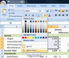
75. Select the cell fill color icon in the Font section of the Home ribbon. Click on the pull-down arrow and select More Colors….
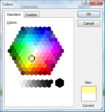
76. Select the third yellow down from the center and click OK.
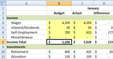
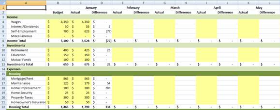
77. Now we’re going to repeat the coloring in all of the sections where a user will edit or enter data – so the Budget column, and each of the Actual columns:
78. Now, we’re going to add some borders to the document. Select cells A4:Z8.
79. 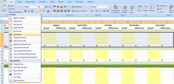
80. Click on the Borders pull down in the Font section of the Home ribbon. Click on All Borders.
81. Now repeat in each section – skipping the colored title rows.
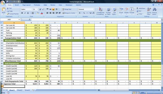
82. We need a Total row at the bottom to add everything up.
83. Click on cell A69.
84. Type in Total and press Enter.
85. Click on cell A69. Change the Indent to 0.
86. Click on row 69. Make it Bold.
87. Select A69:Z69 and set All Borders.
88. Click on the Borders pull down menu and select Top and Double Bottom Border.
89. Click on cell B69.
90. Type in =B8-B13-B68 which calculates the Income Total – Investments – Expenses .
91. Fill the cell to the right across all of the cells to Z69.
92. Select row 2 and click on the Center icon on the Alignment section of the ribbon.
93. Click on cell A1.
94. Select cells A1:Z69 (the entire spreadsheet).
95. Pull down the Borders button menu and select Thick Box Border.
96. Save the spreadsheet.
Congratulations! You have formatted a great spreadsheet!

