Changing Formatting Based on Value, aka Conditional Formatting
One of the features which makes Excel great to use is Conditional Formatting. Conditional Formatting is exactly what it sounds like – changing the formatting of a cell based on a value condition which you specify. For example, you could set a condition that any values above 100 cause the contents of a cell to turn red, while values above 1000 turn the cell green. There are endless possibilities and Excel 2007 makes it much easier to use Conditional Formatting than previous versions.
1. Click on cell D4.
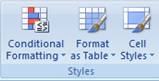
2. Click Conditional Formatting in the Styles section of the Home ribbon.
3. Move your mouse over Highlight Cells Rules.
4. Click on Greater Than.
5. 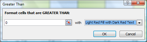
6. Change the value to 0.
7. Click on the pull down menu to the right and select Custom Format.
8. 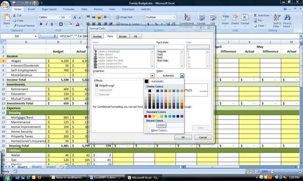
9. Select the dark green color at the bottom of the Color pull down menu on the Font tab. Click OK.
10. Click OK.
11. Now change cell C4 to $4500. Cell D4 changes to Green.
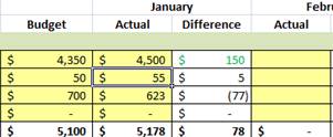
12. Now repeat the process, but this time, select Less Than, change the value to 0 again, and select a format of Red text.
13. Change cell C4 to $4200. Now, the $(150) is red.
14. Using Format Painter, paint the format of cell D4 down column D, skipping the Total cells.
15. We want the format on all of the months – plus we need to paint the $ format on the Actual column to the Actual columns. Select columns C:D.
16. Click on Format Painter twice.
17. Click on columns E:F. Repeat through each set of columns for each month on the spreadsheet.
18. Click Format Painter once to turn it off.
19. Save the spreadsheet.