Working with Formulas
In the previous sections, you have created a pretty budget using a lot of great formatting techniques. In this section, we’re going to start having Excel 2007 do some heavy lifting for us and starting having it perform calculations.
If you’ve skipped ahead or just want to start with a fresh copy of the spreadsheet with where we are at in the tutorial, download it here:
What is a Formula?
An Excel formula is an equation containing functions, cell references, numbers, and/or operators. Excel is very powerful and can perform complex calculations which are updated as easily as entering data in a cell. It has simple functions – such as summing several cells – and much more complex statistical functions.
We’ll focus in the section on the simpler formulas to calculate information we need in our budget.
Creating a Formula
1. Open the Family Budget spreadsheet.
2. Click in cell B8.
3. Click on the ![]() button in the Editing section of the Home ribbon and press Enter:
button in the Editing section of the Home ribbon and press Enter:
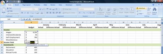
4. The AutoSum button sums the cells which are above and closest to the cell you are in. It stops summing at the first break – in the case, cell B3 has no data, so it is the first break.
5. Click on cell B13. Type in =sum(B10:B12) and press Enter.
6. B10:B12 is a range of cells – it tells Excel to sum all of the cells in the range: B10, B11, and B12.
7. Click on cell B22. Type in =sum(
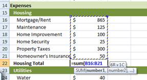
8. Click in cell B16, hold your mouse button down and drag down to cell B21. Press Enter.
9. Now you’ve learned three ways to sum cells – using AutoSum, typing in the cell references directly, and using the mouse.
10. Practice your favorite method by summing each of the “total” rows in the Expenses section.
11. When you get down to cell B68, we will need to use a different method to sum the cells. Since the Expenses section contains a total row in each section, you don’t want to simply sum the entire section or you will be double counting.
12. Click on cell B68. Type in =sum(
13. Go to the top of the Expenses section and click once on cell B22. In the formula bar at the top, you will see it add cell B22 to the formula: ![]()
14. Now hold down the CTRL key and click on cell B32: ![]()
15. Continue the process of holding down the CTRL key and clicking on cells B36, B43, B50, B59, B67:

16. Press Enter.
17. Rows 8 and 13 aren’t bold across all of the cells. Select row 8 and press CTRL+B twice. Repeat with row 13. Why do we have to press it twice? The first cell in the row is already bold, pressing it once unbolds the row, pressing it a second time bolds the entire row.
Great job on entering those formulas! Here’s a copy of the spreadsheet with the formulas in it so you see it before we move on to finishing all of the formulas:
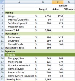
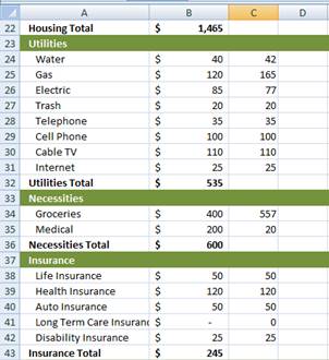
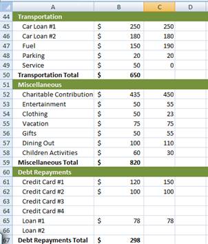
Now, we’re going to enter some data for the month of January so when we create the formulas for each month, it will calculate and we can quickly see if we did it right. Here’s the data we want to enter:
Now, we need to add some more formulas, so let’s get right back into that:
18. Go to cell D4.
19. Type in =C4-B4
20. Press Enter.
21. This formula subtracts cell B4 from cell C4, providing the difference in cell D4.
22. We could go down the spreadsheet and type the formula in each cell but there is a much easier way!
23. Click on cell D4.

24. In the bottom right of the box on cell D4 is a little square box. This is the fill control. There are two ways to use it – click on the small square and drag up, down, right, or left and it will fill those cells with the contents of cell D4.
25. The other way to fill the contents of the cells down is to double-click on the small square in the bottom right of the cell.
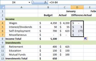
26. This will fill to the first break – the adjacent column C stops at C8, so the D column will automatically fill down to D7, stopping at D8.
27. Earlier, the formula we entered in D4 was =C4-B4, but as you can see on the spreadsheet, each cell is properly calculated the cells to its left – they don’t all have the formula =C4-B4. Excel automatically updates formulas based on where they are copied to – reflecting the intent of the original formula based on its new position. So, for example, it updated the row number for D5 to 5 (so the formula is now =C5-B5), for D6 to 6 and so on.
28. The same update occurs if you copy the formula to a new cell. Click con cell D6 and press CTRL+C to copy the contents of the cell.
29. Click on cell D10 and press Enter.
30. You will notice the formula in cell D10 is updated to reflect its new location.
31. Double-click on the square on the bottom right of the box in cell D10 to fill the contents of D10 down.
32. Now, copy D12 into D16. Fill down the contents of the cell. Repeat this process through all of the sections.
33. Return to the top of the spreadsheet and click on cell B8.
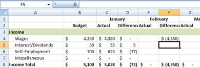
34. We want to fill the formula in this cell across all of the months. Click on the small square in the bottom right-hand side of the cell and hold the mouse button down as you drag it right to cell Z8:

35. Now repeat this process with each of the “total” rows.
36. The C column doesn’t have the proper $ formatting like the other cells. Let’s fix that – click in cell C4.
37. Click the Format Painter button twice.
38. Click and drag down for cells C4:C7. Now repeat in each section which doesn’t have the correct formatting. You do not want to drag all the way down the column or you will unbold the “total” rows.
39. Click the Format Painter button once when you are finished to turn it off.
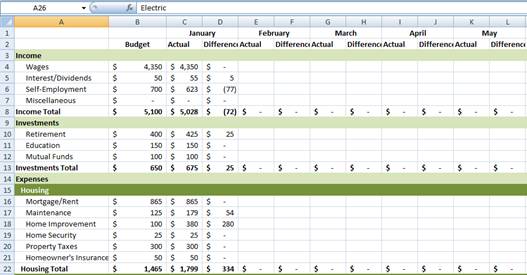
40. Here’s what the spreadsheet looks like so far:
41. Go to cell F4.
42. Type in =E4-B4
43. Press Enter.
44. You may notice a problem here. Though the spreadsheet is accurate – we haven’t earned $4350 yet, so we are negative on wages – but when we use this formula all the way down, the spreadsheet will be a little cluttered – just because the month hasn’t occurred yet. What can we do about it?

