Formatting Your Excel Spreadsheet
In this section of the Microsoft Excel 2007 tutorial, we’re going to continue working with our Family Budget spreadsheet and start really formatting some cells to make the budget stand out.
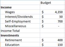
To recap on where we are with the Family Budget: we have designed the framework for the budget, we have started formatting some of the cells, and we’ve entered some numbers in the budget. Here’s a copy of the budget up to this point, in case you have skipped ahead, or if you didn’t want to do all that manual work in the beginning of the tutorial!
Formatting Cells

We need to take this plain vanilla, boring budget and turn it into something easy to read and spectacular!
1. Let’s start by centering the word Budget in cell B1. Click on B1 and click the ![]() icon in the Alignment section of the Home ribbon.
icon in the Alignment section of the Home ribbon.
2. Let’s bold print the cell by clicking the ![]() icon in the Font section.
icon in the Font section.
3. Select row 2.
4. Click on the pull-down arrow on the Fill Color icon ![]() in the Font section of the Home ribbon.
in the Font section of the Home ribbon.
5. Change the color to Olive Green, Accent 3, Lighter 60% (the second light green down). Your row should look this:


6. Now, let’s repeat this process for row 8 (Investments) and row 12 (Expenses).
7. Click on 8 on row 8. Click on the pull-down arrow on the Fill Color icon ![]()
![]()
![]()
![]()
8. Click on 12 on row 12. Click on the pull-down arrow on the Fill Color icon ![]()
![]()
![]()
![]()

