Basic Formatting
Now, still working with Family Budget.xlsx file, let’s start formatting the spreadsheet to make it a little easier to read and work with.
Formatting the Spreadsheet
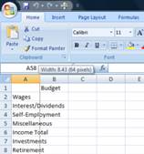
1. The first thing we need to do is to fix the column width of column A to fit all of the categories. There are several ways to enlarge the column, the first way is to manually resize the column using you mouse. Move your mouse to the right edge line of the A column until the cursor changes into a “resize column” cursor:
![]()
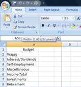
2. You will see the current width appear when you click on the right edge. Now click on the edge and drag to the right, you will see the width change. Release the mouse button and your column will resize.
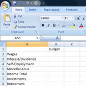
3. An easier way to resize the column automatically to the size of the largest item is to move your mouse to the right edge line of the column label (in this case, the A) and when it turns into a “resize column” cursor, double-click on it. This will resize the column automatically:
4. Now that we have resized the column, let’s start formatting the cells. Our goal is to separate the “title” rows of each section from the labels of the individual budget categories. Let’s start by bolding the title rows.
5. Click on cell A2.
6. Click on the ![]() icon in the Home ribbon or press CTRL+B.
icon in the Home ribbon or press CTRL+B.
7. Now click on cell A7, the Investments cell and click on the ![]()
![]()
![]()
8. Repeat with cells A11, A12, A19, A28, A31, A37, A43, and A51.
9. Now, the A column is a little easier to decipher, but let’s continue formatting to see if we can really make the titles standout.
10. Click on cell A3.
11. 

12. In the Alignment section of the Home ribbon, click on the ![]()
![]()
![]()
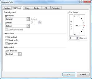

13. In the Indent section of the Alignment tab, click the up arrow twice to set the value to 2: ![]()
![]()
14. Click OK.
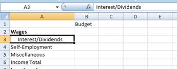

15. Now, Interest/Dividends should be indented. This is a better method of indenting cells versus just inserting two spaces at the beginning of the cell label. If you want to later change this to an indent of “3” or eliminate the indent entirely, you can do that in one simple move. If you had put spaces in each cell manually, this would have been much more difficult.
16. Now, we want to make each of the budget categories indented. You could manually repeat this process on each cell, or you could select several cells and perform this routine on a multiple cells. We’re going to do it a little differently than either of these methods – we’re going to use the format painter.
About the Format Painter
The Format Painter is a great tool in Microsoft Office applications which let’s you apply formatting from a source cell to a different cell.


The Format Painter is available on the Home ribbon in the Clipboard section. There are two ways to use it: a single click allows you to paint the format from one cell to another. Double-clicking the Format Painter allows you to apply the source cell formatting to multiple cells.
17. Click on cell A3.
18. Double-click the Format Painter icon in the Clipboard section of the Home ribbon.
19. Click on cells A4 and then on cell A5.
20. Click once on the Format Painter icon to run off format painting.
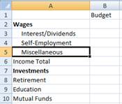

21. Cells A3, A4, and A5 should now have the same indenting.
22. Now, while in cell A5, double-click the Format Painter icon again.
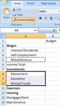

23. Select cells A8 through A10 by clicking your mouse button and holding the mouse button down in cell A8, then drag down to cell A10. Cells A8-A10 will highlight. Release the mouse button and they will be formatted.
24. If at any time you are applying formatting you lose the ability to paint format, click in any cell which is already formatting with indentation and double-click on the Format Painter icon. It’s important to note that whatever cell you are in when you click on the Format Painter icon is the source cell and any cells you click will inherit that cell’s formatting.
25. Now, click on cells A13-A18 to format them with the indentation. Repeat on these groups of cells: A20-A27, A29-A30, A32-A36, A38-A42, A44-A50, and A52-A57.
26. Click on the Format Painter icon to turn format painting off.
27. Now, all of the cells in the spreadsheet should be formatted with the proper indentation to this point. There’s one more set of cells we want to indent – the category titles under the Expenses section.
28. Click on cell A12. Now, we want to select multiple cells which are not next to each other. Hold down the CTRL key on your keyboard and click on cells A19, A28, A31, A37, A43, A51.
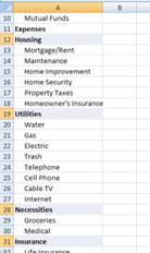

29. You will now have multiple cells selected.
30. Click on the ![]()
![]()
![]()
31. 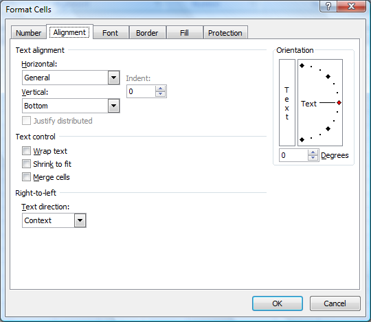

32. Change the Indent section to 1 by clicking on the up arrow.
33. Click OK.
34. All of those labels are now indented by one space.
35. Save the spreadsheet.

