Adding Additional Columns
We need to enter columns for the months of the year so we can compare our budgeted numbers with what we actually spend each month.
First, let’s put in the months. We’re going to put them in every two columns so we have room to enter our actual and then to calculate whether we are over or under budget.
1. Select row 1.
2. Right-click and select Insert. This will insert a new row at the beginning of the spreadsheet.
3. Click on cell C1.
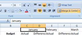
4. Type in January.
5. Now click on cell E1 and type in February.
6. Click on cell G1 and type in March.
7. Repeat this process for each month, skipping one column in between the months, until you have entered December in cell Y1:
![]()
8. Go back to the top left of the spreadsheet and click in cell C2.
9. Type in Actual and press the Tab key.
10. You should now be in cell D2. Type in Difference in cell D2 and press the Tab key.
11. In cell E2, type in Actual, press Tab, then type in Difference in cell F2. Repeat this process for each month:
![]()
12. Don’t worry right now about the size of the columns, we’ll resize all those Difference columns later to make the label fit.
13. Go back to the beginning of the spreadsheet to cell C1.
Centering Column Labels Across Multiple Cells
14. Now we’re going to center the January label over both Actual and Difference.
15. Click in cell C1, hold your mouse button down, and move to the right one cell so both C1 and D1 are selected: ![]()
16. Click on the ![]() button in the Alignment section of the Home ribbon.
button in the Alignment section of the Home ribbon.
17. 
18. The January label is now centered across columns C and D. If you wanted to un-merge and center it, simply click the ![]() button again.
button again.
19. Now, we want to repeat this formatting across each of the months. We’re going to use Format Painter. Click on January, then click on Format Painter twice.
20. Now, select February by clicking in E1, holding the mouse button down, then drag into F1.
21. Repeat with G1 and H1, and so on until all the months are merged and centered over their respective “Actual” and “Difference” columns:
22. When they are all complete, click once on Format Painter to disable it.
![]()
23. Rows 1 and 2 seem important, so let’s bold print them.
24. Select rows 1 and 2 by clicking on 1, holding the mouse button and dragging down one row. Click on the Bold button or press Ctrl+B on the keyboard.
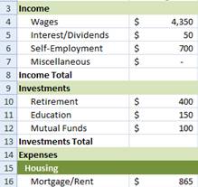
25. We’re missing some “total” lines in each of the sections, so let’s add those now.
26. Right-click on row 13 and click Insert.
27. This will insert a new row 13. Click on cell A13. Type in Investments Total.

28. Cell is indented like the cells above, so we need to reset that formatting.
29. Click on cell A8, press CTRL+B to make the cell Bold.
30. Single click on the Format Painter button. Click on cell A13.
31. Now the cells should be formatted correctly.
32. Right-click on row 22, click Insert.
33. Click on cell A22.
34. Type in Housing Total.
35. Press Enter.
36. Press ALT+H then ALT+F ALT+A. This will open the Alignment dialog box.
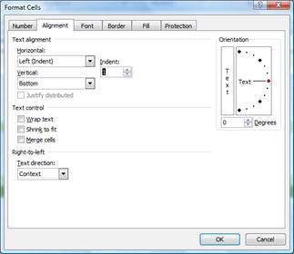
37. Change the Indent to 1. Click OK.
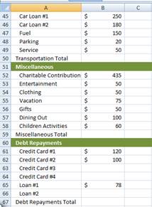
38. Now, repeat this process to add “total” lines to each of the sections in the Expenses section of the spreadsheet.
39. When you get to the bottom, you should be at row 67 for Debt Repayments Total:
40. In row 68, type in Expenses Total and change the Indent to 0.
41. Select row 68 and make it Bold.
42. Go back through and make the “total” rows (row 22, 32, 36, 43, 50, 59, and 67) Bold.
43. Save the spreadsheet.
Congratulations! You have done a great job formatting the document. In the next section, we’re going to explore formulas and start having the spreadsheet perform some calculations for us.